Training and Fine-Tuning Vision Transformers

Next Module →

← Back to Course Menu

Sections

In the evolving world of artificial intelligence, the impact of Vision Transformers (ViTs) on the field of computer vision has been both profound and transformative. Following up on our detailed exploration of the architecture of ViTs in the previous article, this article shifts focus to the practical aspects of training and fine-tuning these powerful models.

Before diving in, if you need help, guidance, or want to ask questions, join our Community and a member of the Marqo team will be there to help.

1. Recap of Vision Transformers

Before we dive into the specifics of training and fine-tuning, let's briefly recap the fundamental aspects of Vision Transformers. Vision Transformers represent a paradigm shift in how machines perceive images, moving away from the conventional convolutional neural networks (CNNs) to a method driven by self-attention mechanisms originally used in processing sequences in Natural Language Processing (NLP).

The core idea behind ViTs is to treat image patches as tokens—similar to words in text—allowing the model to learn contextual relationships between different parts of an image. Each image is split into fixed-size patches, linearly embedded, and then processed through multiple layers of transformer blocks that apply self-attention across the patches. This architecture enables ViTs to capture complex patterns and dependencies, offering a more flexible and potentially more powerful approach to image recognition than traditional methods.

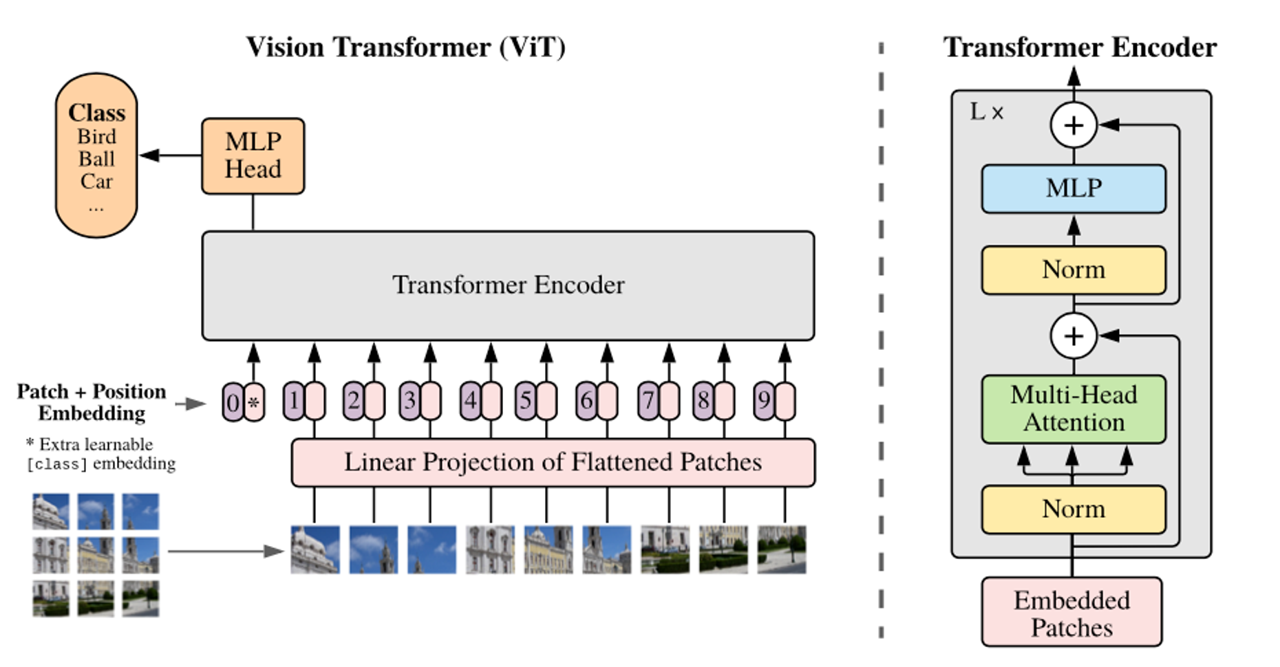
Figure 1: Vision Transformer Model overview: we split an image into fixed-size patches, linearly embed each of them, add position embeddings, and feed the resulting sequence of vectors to a standard Transformer encoder. In order to perform classification, we use the standard approach adding an extra learnable classification token to the sequence [1].

Vision Transformers also scale efficiently with model size and dataset size, often surpassing the performance of CNNs when trained on large-scale datasets. This scalability, combined with their ability to generalize from fewer data when pre-trained on large datasets, makes ViTs a compelling choice for a wide range of vision tasks.

Let’s now take a look at how we can fine-tune our own Vision Transformer for image classification!

2. Fine-Tuning Vision Transformers

In this section, we will discuss how you can leverage Hugging Face’s datasets to download and process image classification datasets and then use them to fine-tune a pre-trained vision transformer (ViT) with Hugging Face’s transformers.

For this article, we will be using Google Colab (it’s free!). If you are new to Google Colab, you can follow this guide on getting set up - it’s super easy! For this module, you can find the notebook on Google Colab here or on GitHub here. As always, if you face any issues, join our Slack Community and a member of our team will help!

Install and Import Relevant Libraries

As always, we need to install the relevant libraries:


!pip install transformers

We will be utilising datasets provided by Hugging Face:


!pip install datasets

Note, when running the following code in this article, some users may be greeted with an error about the accelerate module in Python. To fix this, run:


!pip install transformers[torch] accelerate -U

Amazing! We have installed the relevant modules needed to start fine-tuning.

Load a Dataset

To perform fine-tuning, we will use a small image classification dataset. We’ll use the cats_vs_dogs dataset which is a collection of pictures of cats and dogs. This repository contains custom code so you will have to enter y when prompted to do so after running the code below.


from datasets import load_dataset

ds = load_dataset('cats_vs_dogs')
ds

When we return ds we get the following:


DatasetDict({
    train: Dataset({
        features: ['image', 'labels'],
        num_rows: 23410
    })
})

Notice how the features in the dataset are image and labels. This refers to the image data and the labels associated with each image respectively. Moreover, the num_rows means that we have 23410 rows of data.

Pretty cool! Now, let’s look at an example from the train split from this dataset. We’ll look at the first entry with index 0.


entry = ds['train'][0]
entry

This returns,


 {'image': <PIL.JpegImagePlugin.JpegImageFile image mode=RGB size=500x375>,
 'labels': 0}

We can clearly see the features of the dataset:

image: A PIL Image
labels: A datasets.ClassLabel feature which is given as an integer representation of the label. We may want to translate this into the word (dog or cat) which we’ll do in a moment.

Cool, let’s look at the image!


image = entry['image']
image

This returns the image:

Despite the image being quite blurry, we can easily detect that this is an image of a cat. When we print out the class label for this image, it should return ‘cat’. Let’s look at how we can do that.

First, we want to access the labels feature of the dataset.


labels = ds['train'].features['labels']
labels

This returns,


ClassLabel(names=['cat', 'dog'], id=None)

So, the names of the class label are indeed ‘cat’ and ‘dog’. Let’s obtain the class label for the image above.


labels.int2str(entry['labels'])

Indeed, we get:


'cat'

Nice!

There are so many images of cats and dogs in this dataset so let’s write a function to see a few more with their corresponding labels.


import random
from datasets import load_dataset
import matplotlib.pyplot as plt

# Function to display images with labels in a 3x3 grid
def display_random_images_with_labels(dataset, num_images=9, max_index=23410):
    # Generate random indices
    random_indices = random.sample(range(max_index), num_images)
    
    # Set up the plot
    fig, axs = plt.subplots(3, 3, figsize=(10, 10))
    
    for idx, ax in zip(random_indices, axs.flatten()):
        entry = dataset['train'][idx]
        image = entry['image']
        label_id = entry['labels']
        label_name = dataset['train'].features['labels'].int2str(label_id)
        
        # Display the image
        ax.imshow(image)
        ax.set_title(f'Label: {label_name}', fontsize=10)
        ax.axis('off')
    
    # Adjust layout
    plt.tight_layout()
    plt.show()

# Display 9 random images with their labels in a 3x3 grid
display_random_images_with_labels(ds, num_images=9, max_index=23410)

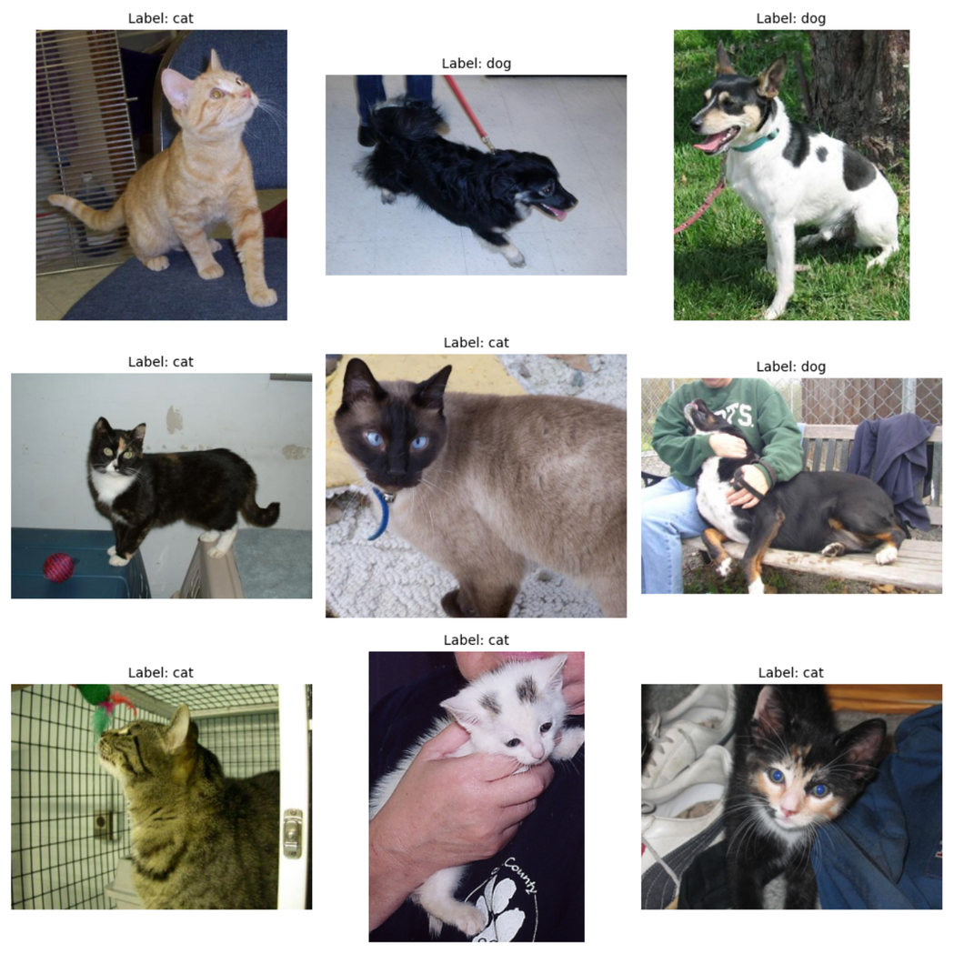
Figure 2: Output from the function defined above. A 3x3 grid containing random samples from the dataset.

As expected, we have images of both dogs and cats. Note, because we’re generating random images, you won’t necessarily see the same images when executing the code yourself.

Awesome, so now we've seen what our dataset looks like, it's time to process this data!

Preparing the Images - ViT Image Processor

We’ve seen what our images look like in this dataset and so, we are in a good position to begin preparing these for our model!

When vision transformers are trained, it’s important to note that the images that are fed into the model must undergo specific transformations. Using the incorrect transformations results in your model not knowing what it’s looking at!

To ensure we apply the correct transformations, we use ViTFeautureExtractor:


from transformers import ViTFeatureExtractor

model_name_or_path = 'google/vit-base-patch16-224-in21k'
vit_feature_extractor = ViTFeatureExtractor.from_pretrained(model_name_or_path)

This code sets up a feature extractor that can preprocess images to be compatible with the google/vit-base-patch16-224-in21k Vision Transformer model.

Let’s take a look at the vit_feature_extractor:


ViTFeatureExtractor {
  "do_normalize": true,
  "do_resize": true,
  "feature_extractor_type": "ViTFeatureExtractor",
  "image_mean": [
    0.5,
    0.5,
    0.5
  ],
  "image_std": [
    0.5,
    0.5,
    0.5
  ],
  "resample": 2,
  "size": 224
}

This JSON object represents the configuration of a ViTFeatureExtractor, which is used to preprocess images for the Vision Transformer (ViT) model. Here's a breakdown of each field:

do_normalize: true
Indicates that the images should be normalized. Normalization typically involves scaling the pixel values to a specific range, often to improve the performance of the neural network.
do_resize: true
Specifies that the images should be resized. Resizing ensures that all images have the same dimensions, which is necessary for batch processing in neural networks.
feature_extractor_type: "ViTFeatureExtractor"
Denotes the type of feature extractor being used, which in this case is ViTFeatureExtractor. This is a specific class designed to preprocess images for Vision Transformer models.
image_mean: [0.5, 0.5, 0.5]
Defines the mean values used for normalization. Each value corresponds to one of the three color channels (Red, Green, and Blue). Normalizing with a mean of 0.5 for each channel means that the pixel values will be centered around 0 when scaled to the range [-1, 1].
image_std: [0.5, 0.5, 0.5]
Defines the standard deviation used for normalization. Each value corresponds to one of the three color channels. Using a standard deviation of 0.5 for each channel means that the pixel values will have unit variance when scaled to the range [-1, 1].
resample: 2
Specifies the resampling filter used when resizing images. A value of 2 typically corresponds to bilinear resampling, which is a common technique for resizing images that maintains a balance between performance and image quality.
size: 224
Indicates the target size of the images after resizing. Images will be resized to 224x224 pixels, which is a standard input size for many Vision Transformer models.

Now, we can process an image by passing it into this vit_feature_extractor.


# Process an image by passing it through the feature extractor
vit_feature_extractor(image, return_tensors='pt')

This will return a dict containing pixel_values which is the numerical representation that needs to be passed to the model. We specify return_tensors='pt' to ensure we get torch tensors instead of NumPy arrays.

Here’s the output:


{'pixel_values': tensor([[[[ 0.5922,  0.6078,  0.6314,  ...]]]])}

We’ve now prepared the images. Let’s look at processing them.

Processing the Dataset

We’ve now covered how you can read and transform images into numerical representations. Let’s combine both of these to process a single entry from the dataset.


def process_single_entry(entry):
    processed = vit_feature_extractor(entry['image'], return_tensors='pt')
    processed['labels'] = entry['labels']
    return processed

The process_single_entry function takes an entry consisting of an image and its label, preprocesses the image using the ViTFeatureExtractor to convert it into a PyTorch tensor, and then attaches the label to the preprocessed image. The final output is a dictionary containing both the preprocessed image tensor and the label, ready to be used for training or inference with a Vision Transformer model. Let’s look at the first entry as an example:


process_example(ds['train'][0])


{
	'pixel_values': tensor([[[[ 0.5922,  0.6078,  0.6314,  ...]]]]),
	'labels': 0
}

Awesome!

We want to do this for every entry in our dataset but this can be slow, especially if you have a large dataset. We can apply a transform to the dataset where it is only applied to entries when you index them.

We will be utilising the function ds.with_transform which expects a batch of data. So, we adjust our process_single_entry function to allow for this.


ds = load_dataset('cats_vs_dogs')

# Function to transform the dataset
def transformation(entry_batch):
    transformed = vit_feature_extractor([x for x in entry_batch['image']], return_tensors='pt')
    transformed['labels'] = entry_batch['labels']
    return transformed

This can now be applied to our dataset using ds.with_transform. First, we must generate our training and validation datasets.

The cats_vs_dogs dataset contains 23410 number of examples. It would be great to fine-tune our existing model on this dataset but for the purpose of the tutorial, we'll create a small subset of this data. Around 1000 training examples and 200 validation examples randomly sampled from the dataset.

Of course, the ideal situation is to have a dataset like beans that is already split into train, validation and test set. However, for the purpose of this tutorial, we wanted to show you how you can fine-tune a dataset that only contains 'train' data.

The code below sets up a reproducible way to split a larger dataset into smaller training and validation subsets using Python’s random module to ensure that the selection of indices is consistent across different runs. The DatasetDict from the Hugging Face datasets library is then used to organize these subsets into a manageable format, facilitating easier access and manipulation during the training and validation processes of our model.


from datasets import DatasetDict
# Set seed for reproducibility
random.seed(42)

# Generate random indices for train and validation datasets
all_indices = list(range(len(ds['train'])))
train_indices = random.sample(all_indices, 1000)
remaining_indices = list(set(all_indices) - set(train_indices))
validation_indices = random.sample(remaining_indices, 200)

# Select the subsets
train_ds = ds['train'].select(train_indices)
validation_ds = ds['train'].select(validation_indices)

# Create a DatasetDict with the new splits
small_ds = DatasetDict({
    'train': train_ds,
    'validation': validation_ds
})

Pretty cool. We now have a smaller dataset with train and validation fields.

We now apply the transform,


# Apply the transformation
prepared_ds = small_ds.with_transform(transformation)

This means that whenever you get an entry from the dataset, the transform will be applied in real time! Take the first two entries for example:


# Take the first two entries for example
prepared_ds['train'][0:2]

The output:


{
	'pixel_values': tensor([[[[ 0.5922,  0.6078,  0.6314,  ...]]]]), 
	'labels': [0, 0]
}

Now the dataset is prepared, let's move onto the training and fine-tuning!

Training and Fine-Tuning

We’re ready to train and fine-tune…almost! Our data is processed and we are in a position to use Hugging Face’s Trainer feature but in order to use this, we must prepare some things.

Data Collator

As we mentioned, we have batches of data which are being inputted as lists of dicts. We need to unpack these.


import torch 

# Data collator function
def collate_fn(batch):
    return {
        'pixel_values': torch.stack([x['pixel_values'] for x in batch]),
        'labels': torch.tensor([x['labels'] for x in batch])
    }

The collate_fn function is used to collate a batch of examples into a single dictionary that can be used by a PyTorch model. It stacks the image tensors into a single batch tensor and converts the list of labels into a tensor. This function is typically passed to the DataLoader to ensure that the data is batched correctly during training or inference.

Evaluation Metric

We want to write a function that takes in the models prediction and computes the accuracy.


import numpy as np
from datasets import load_metric

# Metric computation function
metric = load_metric("accuracy")
def compute_metrics(p):
    return metric.compute(predictions=np.argmax(p.predictions, axis=1), references=p.label_ids)

The compute_metrics function calculates the accuracy of the model's predictions. It does so by:

Converting the model's raw prediction scores into predicted class labels using np.argmax.
Comparing these predicted labels with the true labels (references).
Computing the accuracy using the loaded accuracy metric.

This function is used during the evaluation phase of model training to assess how well the model is performing.

Loading Our Model

We are now in a position to load our pre-trained model. We will also add num_labels to ensure that the model creates a classification head with the right number of units.


from transformers import ViTForImageClassification

# Initialize the model with the correct number of labels
num_labels = len(ds['train'].features['labels'].names)

model = ViTForImageClassification.from_pretrained(
    model_name_or_path,
    num_labels=num_labels
)

Defining Training Arguments

We are one step away from fine-tuning! But, first, we must set up the training configuration by defining TrainingArguments.


from transformers import TrainingArguments

# Training arguments
training_args = TrainingArguments(
  output_dir="./vit-cat-dogs-demo",
  per_device_train_batch_size=16,
  evaluation_strategy="steps",
  num_train_epochs=2,
  fp16=True,
  save_steps=10,
  eval_steps=10,
  logging_steps=10,
  learning_rate=2e-4,
  save_total_limit=2,
  remove_unused_columns=False,
  push_to_hub=False,
  report_to='tensorboard',
  load_best_model_at_end=True,
)

Let’s break down each of these.

output_dir="./vit-cat-dogs-demo":
Specifies the directory where the model checkpoints and logs will be saved during training.
per_device_train_batch_size=16:
Sets the batch size to 16 for each device (e.g., GPU) during training, affecting memory usage and training speed.
evaluation_strategy="steps":
Configures the evaluation to be performed at regular steps rather than at the end of each epoch.
num_train_epochs=10:
Sets the number of epochs (full passes through the training dataset) to 10.
fp16=True:
Enables mixed precision training using 16-bit floating point numbers to speed up training and reduce memory usage.
save_steps=10:
Saves a model checkpoint every 10 steps of training.
eval_steps=10:
Runs evaluation every 10 training steps to monitor model performance.
logging_steps=10:
Logs training metrics (like loss) every 10 steps to provide frequent updates during training.
learning_rate=2e-4:
Sets the learning rate to 0.0002, which controls the step size at each iteration while moving towards a minimum of the loss function.
save_total_limit=2:
Keeps only the most recent 2 checkpoints, deleting older ones to save disk space.
remove_unused_columns=False:
Keeps all columns in the dataset even if they are not used by the model, which can be useful for logging and debugging.
push_to_hub=False:
Disables automatic pushing of the model and logs to the Hugging Face Hub.
report_to='tensorboard':
Configures the training to report metrics to TensorBoard for visualization.
load_best_model_at_end=True:
Loads the best model (according to the evaluation metric) at the end of training for final evaluation and potential deployment.

Let’s Start Training!

We utilise Trainer and pass relevant fields:


from transformers import Trainer
# Initialize the Trainer
trainer = Trainer(
    model=model,
    args=training_args,
    data_collator=collate_fn,
    compute_metrics=compute_metrics,
    train_dataset=prepared_ds["train"],
    eval_dataset=prepared_ds["validation"],
    tokenizer=vit_feature_extractor,
)

Let’s break down the entries:

model=model:
Specifies the model to be trained or evaluated, which is passed to the Trainer.
args=training_args:
Provides the training configuration and hyperparameters defined in the TrainingArguments object.
data_collator=collate_fn:
Uses the collate_fn function to batch process the data correctly during training and evaluation.
compute_metrics=compute_metrics:
Sets the function to compute evaluation metrics, which helps in assessing model performance.
train_dataset=prepared_ds["train"]:
Specifies the training dataset to be used for training the model.
eval_dataset=prepared_ds["validation"]:
Specifies the validation dataset to be used for evaluating the model during training.
tokenizer=vit_feature_extractor:
Uses the vit_feature_extractor for preprocessing the input images, ensuring they are correctly formatted for the model.

Let’s Run the Fine-Tuning!

All that’s left to do is to run the fine-tuning.


# Train the model
train_results = trainer.train()
trainer.save_model()
trainer.log_metrics("train", train_results.metrics)
trainer.save_metrics("train", train_results.metrics)
trainer.save_state()

Here’s the output:

Figure 3: Output from our fine-tuning script.

Now, there's a few things we need to talk about here. Let's first discuss the results from the fine-tuning.

These fine-tuning results showcase several important trends and behaviors in the model's learning process over time:

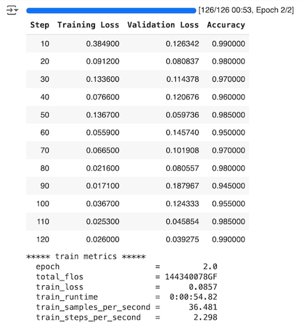
Training Loss: The training loss generally shows a declining trend as the steps increase, which is an encouraging sign of the model learning and improving from the training data. Notably, the training loss decreases substantially from the initial to the final step, with occasional upticks (such as at steps 30 and 50), which could be due to the model adjusting to complexities or nuances in the dataset.
Validation Loss: The validation loss shows more variability compared to the training loss. It starts low, increases at certain points (notably at step 90, reaching the peak), and then decreases again. This pattern suggests that the model might be experiencing some challenges in generalizing to unseen data at certain training stages, particularly around step 90.
Accuracy: The accuracy of the model on validation data starts very high at 99% at step 10 and fluctuates with a general decreasing trend up to step 90, where it drops to its lowest at 94.5%. However, it recovers well towards the end, returning to 99% at step 120. The high starting accuracy could suggest that the model was already quite effective even at early fine-tuning stages, possibly due to pre-training on a similar task or dataset.
Potential Overfitting: At step 90, where the validation loss is at its highest and accuracy is at its lowest, the model is likely experiencing overfitting. This is indicated by a low training loss coupled with high validation loss and reduced accuracy.
Overall Trends: The final steps (110 and 120) show an optimal balance with low validation loss and high accuracy, suggesting that the model has achieved a good generalization capability by the end of this fine-tuning phase. This is an encouraging sign that the fine-tuning process has successfully enhanced the model's performance on the validation dataset.

It's important to note that the dataset we choose when fine-tuning is random and so the results you get from running this Google Colab script will not be the same every time.

Looking at the output above, you will notice that the underlying model actually initially performs really well. At step 10, we have an accuracy of 99%! So, fine-tuning for this dataset isn't necessarily needed, depending on what random sample of pictures are generated in the test and validate sets. Of course, if you were to change your dataset to something our base model, google/vit-base-patch16-224-in21k, wasn't well suited for then you may see drastic improvements in the fine-tuning process.

We selected this dataset because it's important to be aware of different trends that may happen when fine-tuning:

High Variance in Validation Metrics: If you observe significant fluctuations in validation loss or accuracy, as compared to more stable or consistently improving training metrics, it might indicate that the model is fitting too closely to the training data and not generalizing well to new data.
Disparity Between Training and Validation Loss: If the training loss continues to decrease while the validation loss starts to increase, it's a classic sign of overfitting. A low training loss accompanied by a high validation loss generally indicates overfitting.
Complexity of the Model: Larger models with more parameters are more prone to overfitting because they have the capacity to learn extremely detailed patterns in the training data. This can be problematic if those detailed patterns do not apply to new data.
Insufficient Training Data: Overfitting is more likely when the model is trained on a small dataset. A model trained on a limited amount of data might not encounter enough variability to generalize well to unseen data.

Why don't you try out different datasets yourself and let us know what results you get in our Community channel!

3. Conclusion

In this article we’ve expanded on our knowledge of Vision Transformers and performed fine-tuning to a base model for image classification. In the next article, we’ll be taking a look at multi-modal embedding models such as CLIP; diving into how they work and how they can also be fine-tuned!